Greenbar Formatting In Excel
May 21, 2002 - by Bill Jelen
If you are over a certain age, you will remember when all computer reports were produced by the MIS department using COBOL and a high-speed IBM Line Printer. These reports always printed on paper called "Greenbar". Four rows were shaded in green, then four rows were shaded in white. These reports had 132 characters across, and being able to follow the colors across helped you to keep your place on the report.
Using Greenbar formatting in Excel has a nice retro look. It is also still easier to follow the lines across the page. This article will discuss three options for applying greenbar formatting to a report.
Method 1
Use AutoFormat
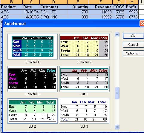
- Start with data in a list format.
- Select any cell in the list.
- From the menu, select Format - AutoFormat
- In the AutoFormat dialog, you will see 6 formats. Use the scrollbar to slide down to the third page of formats. Select the format called List2. Click OK.
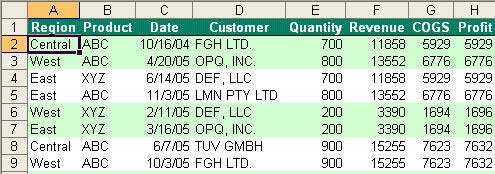
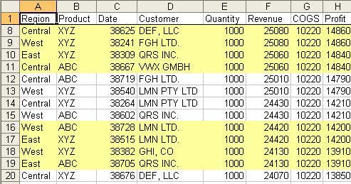
Excel will apply a greenbar effect as shown:
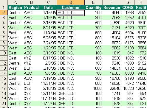
The disadvantage of this method is that as you sort the data, the formatting travels with the original row. After sorting the above data by customer, the nice pattern of 2-green followed by 2-white is a haphazard pattern of green and white:
Method 2
Use Conditional Formatting

- Select all the cells in your list.
- From the menu, select Format > Conditional Format
- In the Conditional Format dialog, change the first dropdown from "Cell Value Is" to "Formula Is".
- Enter this formula in the Formula box:
=MOD(ROW(),2)=0 - Click the Format... button
- In the Format Cells dialog, Click the Patterns tab
- Choose a light green (or light blue or light yellow) pattern. Click OK.
- Click OK to close the Conditional Formatting dialog
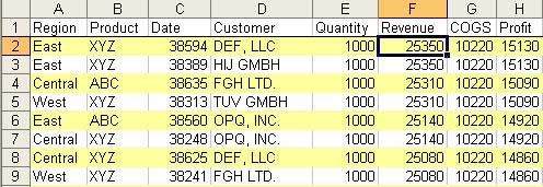
The result will be a greenbar effect with every other row highlighted. It is created by conditional formatting. You are free to re-sort the data, delete rows or even insert rows in the middle of the data. The greenbar formatting effect will persist.
The formula in the Conditional Formatting box uses the MOD function. Do you remember when you were first learning how to do long division? If you had to divide 7 into 25, you might come up with the answer of "3 with a Remainder of 4"? The MOD function tells you the remainder after doing the division. So, =MOD(25,7) would be 4 - because the remainder after 7 goes into 25 is 4.
In the conditional formatting above, you divided the row number by 2. If the remainder was 0, then it is an even numbered row and the conditional format pattern was applied.
It is possible to experiment with the formula to create alternate banding patterns. For example, divide the row number by 8. If the remainder is 0 through 3, use a green pattern. Otherwise, use the white pattern. Here are some sample formulas:
- 2 Green followed by 2 white:
=MOD(ROW(),4)<2 - 3 Green followed by 3 white:
=MOD(ROW(),6)<3 - 4 Green followed by 4 white:
=MOD(ROW(),8)<4
Method 3
Use a VBA Macro
The above method fails if you have hidden rows in your data. This is common if you are using an AutoFilter or Group and Outline Mode. Method 2 can not be used if you already have conditional formatting in your data. In this case, the solution is the following macro. If you are not familiar with the Visual Basic Editor, read Introducing the Excel VBA Editor.
Enter the following code on a standard module:
Sub ApplyGreenBarToSelection()
    n = 0
    For Each VisRow In Selection.Resize(, 1).SpecialCells(xlCellTypeVisible)
        n = n + 1
        If n Mod 2 = 0 Then
            VisRow.EntireRow.Interior.ColorIndex = 35
        End If
    Next VisRow
End Sub
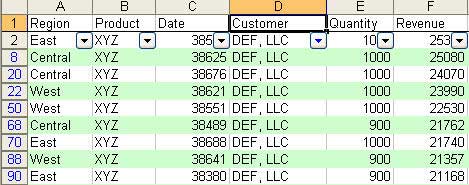
In the image below, I've turned on the AutoFilter feature and filtered to just the records for Customer DEF. Select all of the cells in the selection and use Tools - Macro - Macros to run ApplyGreenBarToSelection.
The key to this VBA macro is the .SpecialCells method.
