Gantt Chart With Conditional Formatting
May 14, 2002 - by Bill Jelen
Phil wrote this morning asking about creating chart in Excel.
Is there any way to take two columns holding start and stop dates for individual events and create a Gantt type chart without having to leave Excel?
This topic was covered in the Create Timeline Chart tip. That tip from the summer of 2001 mentioned that you could also create a Gantt-type chart on a worksheet using conditional formatting. This type of chart would solve Phil's question.

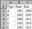
I imagine that Phil's data looks something like the table to the left. There is an event, then start dates in column B and end dates in column C. I am using years for my example, but you could easily use regular Excel dates.
The next step could easily be incorporated into a macro, but the real focus of this technique is setting up the conditional formatting. I scanned through my data and noticed that the dates range from 1901 to 1919. Starting in column D, I entered the first year 1901. In E1, I entered 1902. You can then select D1:E1, click on the fill handle in the lower right corner of the selection with your mouse and drag out to column W to fill in all of the years from 1901 to 1920.
In order to make the years take up less room, select D1:W1, then using Format - Cells - Alignment, select the vertical text option. Then select Format - Column - Autowidth and you will be able to see all 23 columns on the screen.

Select the upper left cell of the Gantt chart area, or D2 in this example. From the menu, select Format - Conditional Formatting. The dialog box initially has a drop down on the left side that defaults to "Cell Value Is". Change this dropdown to "Formula Is" and the right side of the dialog box will change to a large textbox for entering a formula.
The goal is to enter a formula that checks to see if the year in row 1 above this cell falls within the ranges of years in columns B & C of this row. It is important to use the right combination of relative and absolute addresses so that the formula we enter in D2 can be copied to all of the cells in the range.
There will be two conditions to check and both will have to be true. This means that we are going to start with the =AND() function.
The first condition will check to see if the year in Row 1 is greater than or equal to the year in column B. Since I always want this formula to refer to row 1, the first part of the formula is D$1>=$B2. Note that the dollar sign before the 1 in D$1 will insure that our formula always points to row 1 and that the dollar sign before the B in $B2 will insure that it always compares to column B.
The second condition will check to see if the year in Row 1 is less than or equal to the date in column C. We still need to use the same relative & absolute addressing, so this will be D$1<=$C2
We need to combine both of those conditions using the AND() function. This would be =AND(D$1>=$B2,D$1<=$C2)
In the formula box of the Contional Formatting dialog, enter this formula. Make sure to start with an equal sign or the conditional formatting will not work.
Next, choose a bright color to be used whenever the condition is true. Click the Format... button. On the Patterns tab, select a color. Click OK to close the Format Cells dialog and you should be left with a Conditional Formatting dialog that looks like this one

Click OK to dismiss the Conditional Formatting box. If your upper left cell in D2 happens to fall in a year, that cell will turn yellow.
Whether the cell turned yellow or not, click on D2 and use Ctrl + C or Edit - Copy to copy that cell.
Highlight D2:W6 and from the menu select Edit - PasteSpecial - Formats - OK. The conditional format will be copied to the entire range of the Gantt Chart and you will end up with a chart that looks like this one.

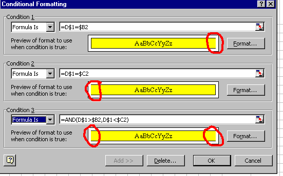
Conditional formatting is a great tool and lets you easily create Gantt-type charts right on the worksheet. Keep in mind that you are limited to only three conditions for any cell. You can experiment with different combinations of conditions. In order to create borders around each bar in the Gantt chart, I used three condtions as shown below and used different borders for each condition.


