
Fill Pivot Blank Cells
April 30, 2002 - by Bill Jelen
This tip is an extension of last week's Excel tip. You can use the Go To Special command to select the blank cells from a range. This is great Excel technique for cleaning up data in a pivot table.
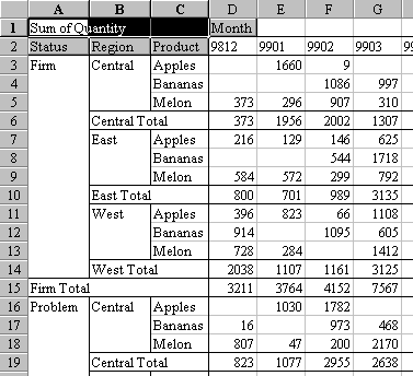
Pivot tables are wonderful tools. But what if your pivot table is just an intermediate step in your data manipulations and you want to make further use of the summarized data in the pivot table? I used to regularly receive 5000 rows of data from a legacy mainframe system. This data has columns for product, month, region, status and quantity. I needed to summarize the data in a pivot table with months going across the top, product, region and status going down the rows. Pivot tables make this a snap.
From there, I needed to take the data from the pivot table and import to Access. As you can see, the default pivot table is not suitable for this. Excel uses a outline style so that each region appears only once, with blank cells following it until the Region Subtotal. Cells in the data section without data are blank instead of numeric. I also do not want the subtotals in the data.
Starting in Excel 97, there are options for the pivot table to control some of this behavior.
In the Pivot Table layout dialog, double click the field name for region. In the Subtotals section, click the radio button for "None". This will get rid of the unwanted subtotals.
In Excel 2000, the options button will take you to a dialog where you can specify "For empty cells, show:" and fill in a zero so that you do not have a table full of blank cells.
To further manipulate the pivot table, you will have to make it no longer be a pivot table. If you try and change cells in a pivot table, Excel will tell you that you can not change part of a pivot table. To change from a pivot table to just values, follow these steps:
- Move the cell pointer outside of the pivot table.
- If the pivot table starts on row 1, then insert a new row 1.
- Start highlighting in the new blank row 1 and drag down to select the entire pivot table.
- Do Ctrl + C (or Edit - Copy) to copy this range.
- With the same area selected, do Edit - Paste Special - Values - OK to change the pivot table to just static value.
But here is the real tip for this week. Jennifer writes
I have continually run into the problem of using the pivot table option, to summarize reams of data, but it does not fill in the rows beneath each change in row category. Do you know how to make the pivot table fill in below each change in category?? I have been having to drag and copy every code down so I can do more pivot tables or sorting. I have tried changing the options in the pivot table, to no avail.
The answer is not easy to learn. It is not intuitive. But, if you hate dragging those cells down, you will love taking the time to learn this process! Follow along - it seems long and drawn out, but it really really works. Once you get it, you can do this in 20 seconds.
There are actually 2 or 3 new tips here. Let's say you have 2 columns on the left which are in outline format that need to be filled in. Highlight from cell A3 all the way down to cell B999 (or whatever your last row of data is.)
Trick #1. Selecting all of the blank cells in that range.
Hit Ctrl + G, Alt + S + K and then enter. huh?
Ctrl + G brings up the GoTo dialog
Alt + S will pick the "Special" button from the dialog box
The Goto-Special dialog is an awesome thing that few know about. Hit "k" to pick "blanks". Hit enter or click OK and you will now have selected just all of the blank cells in the pivot table outline columns. These are all of the cells which you want to fill in.
Trick #2. Don't watch the screen while you do this - it is too scary and confusing.
Hit the equals key. Hit the Up arrow. Hold down Ctrl and hit enter. Hitting equals and the up arrow says, "I want this cell to be just like the cell above me." Holding down Ctrl when you hit enter says, "Enter this same formula in every selected cell, which, thanks to Trick #1 is all of the blank cells which we wanted to fill in.
Trick #3. Which Jennifer already knows, but is here for completeness.
You now need to change all of those formulas to values. Select all of the cells in A3:B999 again, not just the blanks. Hit Ctrl + C to copy this range. Hit Alt + E then sv (enter). to Paste Special Values these formulas.
Ta-da! You will never spend an afternoon manually pulling down column headings in a pivot table again.