Duplicates With Conditional Formatting
January 08, 2002 - by Bill Jelen
Last night on Craig Crossman's Computer America radio show, Joe from Boston had a question:
I have a column of invoice numbers. How can I use Excel to mark the duplicates?
I suggested using conditional formats and the COUNTIF formula. Here are the details on how to make that work.
We want to set up conditional formatting for the whole range, but it is easier to set up a conditional format for the first cell in the range and then copy that conditional format. In our case, cell A1 has a heading of invoice number, so I will select cell A2 and from the menu, select Format > Conditional Formatting. The Conditional Formatting dialog starts with the initial dropdown saying "Cell Value Is". If you touch the arrow next to this, you can choose "Formula Is".

After selecting "Formula Is", the dialog box changes appearance. Instead of boxes for "Between x and y", there is now a single formula box. This formula box is incredibly powerful. You can type in any formula that you can dream up, as long as that formula will evaluate to TRUE or FALSE.
In our case, we need to use a COUNTIF formula. The formula to type in the box is
=COUNTIF(A:A,A2)>1
In English, this says, "look through the entire range of column A. Count how many cells in that range are the same value as what is in A2. (It is really important that the "A2" in the formula be pointing to the current cell - the cell that you are setting the conditional formatting up in. So - if your data is in column E and you are setting the first conditional formatting up in E5, the formula would be =COUNTIF(E:E,E5)>0). Then, we compare to see if that count is > 1. Ideally, with no duplicates, the count will always be 1 - because cell A2 is in the range - we should find exactly one cell in column A that contains the same value as A2.
Click the Format... button


Now it is time to select an obnoxious format. There are three tabs across the top of this Format Cells dialog. The Font tab is usually first, so you could select a Bold, red font, but I like something more obnoxious. I usually click the Patterns tab and choose either bright red or bright yellow. Choose the color, then click OK to close the Format Cells dialog.
You will see the selected format in the "Preview of format to use" box. Click OK to close the Conditional Formatting dialog...
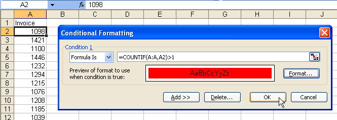
...and nothing happens. Wow. If this is your first time setting up conditional formatting, it would be really nice to get some feedback here that it worked. But, unless you are lucky enough that the 1098 in cell A2 is a duplicate of some other cell, the condition is not true, and it looks like nothing happened.
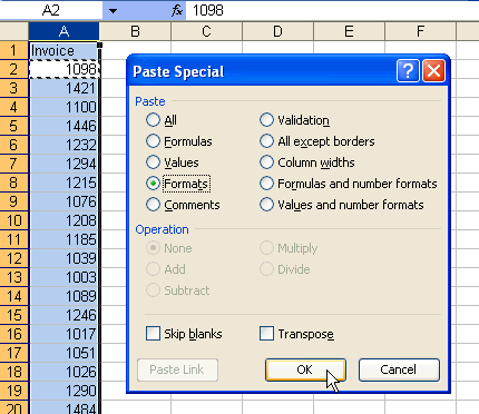
You need to copy the conditional formatting from A2 down to the other cells in your range. With the cursor sill in A2, do Edit > Copy. Hit Ctrl + Spacebar to select the entire column. Do Edit > Paste Special. In the Paste Special dialog, click Formats. Click OK.
This will copy the conditional formatting to all cells in the column. Now - finally - you see some cells with the red formatting, indicating that you have a duplicate.
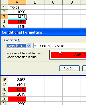
It is informative to go to cell A3 and look at the conditional format after the copy. Select A3, hit od to bring up conditional formatting. The formula in the Formula Is box as changed to count how many times A3 appears in the column A:A.
Notes
In Joe's question, he only had 1700 invoices in the range. I've set up 65536 cells with conditional formatting and each cell is comparing the current cell to 65536 other cells. In Excel 2005 - with more rows - the problem will be even worse. Technically, the formula in the first step could have been: =COUNTIF($A$2:$A$1751,A2)>1
Also, when copying the conditional format to the entire column, you could have instead selected just the rows with data before doing the Paste Special Formats.
More
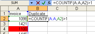
The other issue that I described after the question is that you really can not sort a column on the basis of a conditional format. If you need to sort this data so that the duplicates are in one area, then follow these steps. First, Add a heading to B1 called "Duplicate?". Type this formula in B2: =COUNTIF(A:A,A2)>1.

With the cell pointer in B2, click the autofill handle (the little square in the lower right corner of the cell) to copy the formula all the way down the range.
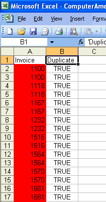
You can now sort by column B descending and A ascending to have the problem invoices at the top of the range.
This solution assumes that you want to highlight BOTH of the duplicate invoices so that you can manually figure out which to delete or correct. If you don't want to mark the first occurence of the duplicate, you can adjust the formula to be: =COUNTIF($A$2:$A2,A2)>1. It is important to enter the dollar signs exactly as shown. This will look at all cells from the current cell up only, looking for duplicate entries.
Thanks to Joe from Boston for the question!
